Introduction
In the ever-evolving landscape of artificial intelligence (AI), researchers and developers are constantly striving to create more efficient and powerful neural networks. One promising avenue in this pursuit is Neural Architecture Search (NAS), a groundbreaking technique that holds the potential to revolutionize the way we design and optimize deep learning models. In this blog, we will delve into the world of NAS and explore how it is shaping the future of AI.
What is Neural Architecture Search?
Neural Architecture Search is a process that automates the design of neural networks. Traditionally, developing an effective neural network required a great deal of manual trial and error, with researchers spending countless hours fine-tuning the architecture to achieve optimal performance. NAS aims to eliminate this time-consuming process by employing computational methods to automatically discover the best network architecture for a given task.
The Process
The process of Neural Architecture Search involves training and evaluating numerous candidate architectures to identify the most effective one. It typically begins with a search space, which defines the set of possible architectures that the NAS algorithm will explore. This search space can range from simple choices such as the number of layers and the size of each layer, to more complex decisions such as the type of activation function or the presence of skip connections.
To efficiently navigate through this vast search space, various techniques are employed. These include reinforcement learning, evolutionary algorithms, gradient-based optimization, and Bayesian optimization. These methods aim to strike a balance between exploration (searching for new promising architectures) and exploitation (improving the performance of already discovered architectures) to find the optimal neural network design.
Search Procedure
1. Create random population (architectures).
2. Crossover between population.
3. Mutation on crossover population.
4. Find the fittest population from previous and crossovered population.
5. Repeat above three steps for multiple times for better architectures.
Initialization of population
➜ Each neural network architecture is sub divided into phases.
➜ No phases in an architecture is predefined.
➜ Each phase contains 'n' number of nodes.
➜ Each node represents a convolution or dense layer.
➜ Each phases are connecting from its previous phase by downsampling outputs of its previous phase.
➜ Evolution of network topology happens by varying connections between nodes.
Representation of phase
Each phase consists of 'n' no. of nodes and the connection between these nodes are represented as binary string. The nodes within each stage are ordered, and we only allow connections from a lower-numbered node to a higher numbered node. Each node corresponds to a convolutional operation, which takes place after element-wise summing up all its input nodes (lower-numbered nodes that are connected to it).
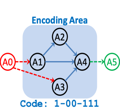
Reference: https://arxiv.org/pdf/1810.03522.pdf
Inputs and outputs of phases are not encoded. From the diagram on the left, nodes in blue are only encoded. We can see that A2 is connected to A1, so first bit is 1.
A3 can have connection from A1 and A2, so to represent A3 connection 2 bits are needed. A3 is not connected to A1 and A2, so both bits are 0.
Similarly A4 has 3 connections where it has all the connection from its previous nodes so all of bits are 1.
Homogeneous Crossover
Homogeneous crossover operator takes two selected population members as parents, to create offspring (new network architectures) by inheriting and recombining the building-blocks from parents.
The main idea of this crossover operator is to preserve the common building-blocks shared between both parents by inheriting the common bits from both parent's binary bit-strings.
Maintain relatively, the same complexity between the parents and their offspring by restricting the number of "1" bits in the offspring's bit-string to lie between the number of "1" bits in both parents.
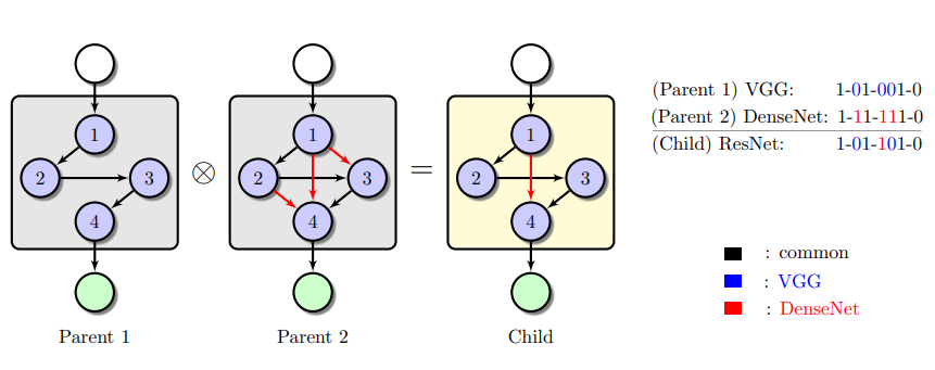 Reference: https://arxiv.org/pdf/1810.03522.pdf
Parent 1 phase has connection between their nodes in vggfashion where each node is connected to only its immediate precursor node.
Parent 2 phase has connections resembling to dense block of dense net architecture.
Cross over operation reserved the bits which have same bit encoding and remaining bits of child are chosen with random sampling.
Mutation
To enhance the diversity (having different network architectures) of the population and the ability to escape from local optima, a bit-flipping mutation operator is used, which is commonly used in binary-coded genetic algorithms.
Due to the nature of our encoding, a one bit flip in the genotype space could potentially create a completely different architecture in the phenotype space. Hence, we restrict the number of bits that can be flipped to be at most one for each mutation operation. As a result, only one of the phase architectures can be mutated at one time.
Selection
Fitness Function : Accuracy of child architecture is measured as fitness of individual architecture. Accuracy and the model size are considered as multi objectives which algorithm tries to optimize.
Selection Flow :
1. Get accuracies and model size of both parents and cross over population from a generation.
2. Divide the population into fronts.
3. By using crowding distance survival method select top n fronts from overall population at that particular generation.
Fronts
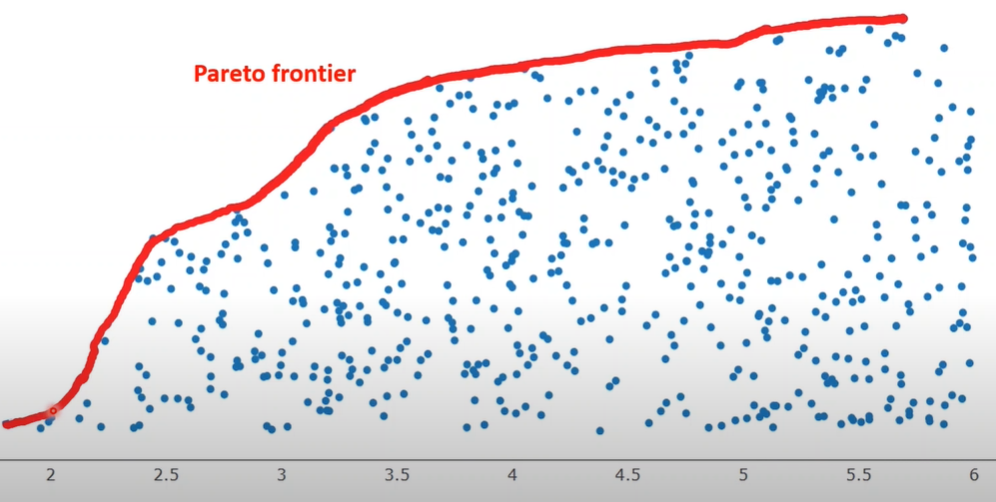
Reference: https://www.youtube.com/watch?v=SL-u_7hIqjA&t=257s
Figure from left represents two objectives plot with y scale objective needs to be maximized and x scale objectives needs to be minimized.
Blue points represents objective values obtained from fitness functions of populations.
Red line represents front where each population on front has no better solution as moving in either direction will reduce one of the objective values in the population space.
Finding Pareto optimal Fronts(Non Dominated Sorting)
Plot on the right shows two objective values which we need to minimize.
Green ,blue and red represent fronts they belong to.
For assigning a particular individual to a front domination count and individuals which were dominated by this individual are required.
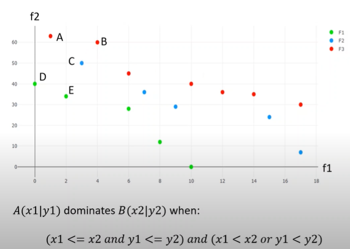
Reference: https://www.youtube.com/watch?v=SL-u_7hIqjA&t=257s
To say an individual P dominated individual Q both fitness values should of P should be less than or equal to Q fitness values and at least one of the fitness values of P should be less than Q fitness values in minimization problem.
Once domination counts of all individuals are retrieved ,individuals having 0 domination count meaning which didn't get dominated by any individuals are assigned to front 1.
For assigning other individuals to front 2 .individuals which were dominated by front 1 individuals are considered and we reduce these individuals domination count.
By the end of this iteration we find new individuals which has domination count 0. These individuals will be assigned to front 2. Like was all other individuals will be assigned to all other fronts.
Crowding source distance sorting
Once the individuals are assigned to fronts, rank is given to the each individuals according to their fronts. Individuals in front 1 will have rank 1 likewise for other individuals. Once individuals are ranked, only some of the individuals gets selected for next generation. Some of the Least ranked front individuals gets discarded.
Individuals in least rank front are assigned crowding distance score. Individuals which high scores gets picked first. Score is calculated by sorting fitness values of objectives, individuals having highest and lowest fitness values are given score infinity.
For rest of individuals score is calculated by taking difference of immediate large value fitness and immediate less values fitness scores and dividing it by difference of maximum fitness score and least fitness score in that front. This way of selection helps in creating diversity in population.
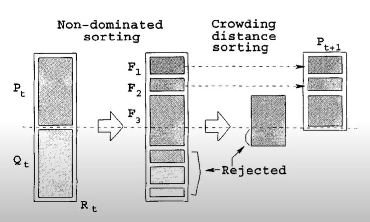
Reference: https://www.youtube.com/watch?v=SL-u_7hIqjA&t=257s
NSGA II Flow :
➜ Create n architectures randomly.
➜ Calculate accuracies and model sizes of architectures.
➜ Make crossover and mutation between architectures.
➜ Divide the architecture into fronts with non dominated sorting .
➜ Rank the fronts and select n population from above population using crowding distance sorting.
➜ Repeat the above steps for multiple generations.
Experiment :
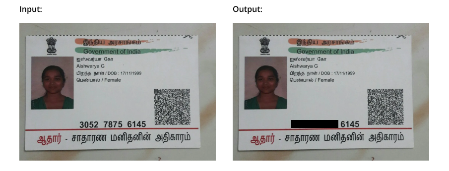
Implemented nsga II for detection of aadhaar numbers in aadhar card. Whole algorithm ran for 14 days with 7 generations. Replaced darknet with nas genes and each child architecture was trained from scratch without any transfer learning. Below table represents results of nas object detection models vs standard yolo model.
| # | Test sets | YOLO(250 MB) | NSGA II(30 MB) |
|---|---|---|---|
| 1 | Test set 1 | 100 | 99 |
| 2 | Test set 2 | 100 | 99 |
| 3 | Test set 3 | 100 | 100 |
| 4 | Test set 4 | 100 | 99 |
| 5 | Test set 5 | 94 | 95 |
| 6 | Test set 6 | 95 | 93 |
| 7 | Test set 7 | 96 | 97 |
NSGA II results for Aadhar masking
Conclusion :
In conclusion, Neural Architecture Search is at the forefront of AI research offering a path to unlock the full potential of deep learning. By automating the design of neural networks, NAS holds the promise of significantly improving performance, reducing time and cost, and enabling breakthroughs in various domains. As researchers continue to refine and expand NAS techniques, we can anticipate a future where AI systems are not only more powerful but also more accessible and efficient. The journey towards fully automated neural network design has just begun, and the possibilities are endless.